Resumen
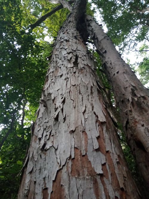
El presente estudio consiste en una aproximación biogeográfica de la especie Brosimun alicastrum SW, retomando su respectiva distribución en países de América Latina. Es considerada como una especie multipropósito, adquiere su funcionalidad a partir del uso y técnicas de aprovechamiento en distintas comunidades. Se pretende análisar la distribución actual del ojoche y aproximarse al aprovechamiento que genera esta especie a nivel a las comunidades y soberanía alimentaria.
(Brosimum alicastrum)

Metodología
El estudio se basa en los datos del Sistema Global de Información sobre Biodiversidad GBIF red internacional e infraestructura de datos financiada por los gobiernos del mundo para dar a cualquiera, en cualquier lugar, acceso abierto a datos sobre todas las formas de vida en la Tierra.
Los datos son parte del trabajo colaborativo con registros de la población de las comunidades vinculada o consciente de integrar la información, para un total de 14220 de especies de ojoche encontradas.
Distribución geográfica
In [ ]:
pip install tabulate
Requirement already satisfied: tabulate in /usr/local/lib/python3.11/dist-packages (0.9.0)
Aprovechamiento del Ojoche
| Aprovechamiento | Estructura |
|---|---|
|
1. Follaje. 2. Medicina. 3. Alimentos. |
Hojas, semillas. Semillas, corteza,latex. Agua. |
Variedades de ojoche
In [ ]:
# Import the tabulate module
from tabulate import tabulate

# Sample data: list of lists
data = [
    ["Reino", "Plantae"],
    ["Filo", "Tracheophyta"],
    ["Clase", "Magnoliopsida"]
]

# Creating a table with headers and a grid format
table = tabulate(
    data,
    headers=["Clasificación", "NOmbre"],
    tablefmt="grid"
)

print(table)
+-----------------+---------------+
| Clasificación   | NOmbre        |
+=================+===============+
| Reino           | Plantae       |
+-----------------+---------------+
| Filo            | Tracheophyta  |
+-----------------+---------------+
| Clase           | Magnoliopsida |
+-----------------+---------------+
In [ ]:
import geopandas as gpd
In [ ]:
# Carga de pandas con el alias pd
import pandas as pd

# Carga de folium
import folium

# Carga de matplotlib
import matplotlib.pyplot as plt
In [ ]:
# Biblioteca requerida para mapas interactivos
!pip install mapclassify --quiet

import mapclassify
In [ ]:
# Montaje de Google Drive en Colab
from google.colab import drive
drive.mount('/content/drive')
Drive already mounted at /content/drive; to attempt to forcibly remount, call drive.mount("/content/drive", force_remount=True).
In [ ]:
# Carga de un archivo CSV desde Google Drive
ojoche = pd.read_csv(
    "/content/drive/MyDrive/Colab Notebooks/ojoche.csv",
    sep="\t"
)
# Despliegue de los últimos registros
ojoche.tail(10)
Out[ ]:
| gbifID | datasetKey | occurrenceID | kingdom | phylum | class | order | family | genus | species | ... | identifiedBy | dateIdentified | license | rightsHolder | recordedBy | typeStatus | establishmentMeans | lastInterpreted | mediaType | issue | |
|---|---|---|---|---|---|---|---|---|---|---|---|---|---|---|---|---|---|---|---|---|---|
| 14197 | 1038454392 | 99b1c33f-113b-4477-8075-a9bbe5df0246 | IAvH:BICUB:MAGNOLIOPHYTA:OBSERVACIONHUMANA:I2D... | Plantae | Tracheophyta | Magnoliopsida | Rosales | Moraceae | Brosimum | Brosimum alicastrum | ... | NaN | NaN | CC_BY_NC_4_0 | UTP | Dorian Ruiz Penagos | NaN | NaN | 2025-02-06T18:17:13.282Z | NaN | GEODETIC_DATUM_ASSUMED_WGS84;CONTINENT_DERIVED... |
| 14198 | 1038454387 | 99b1c33f-113b-4477-8075-a9bbe5df0246 | IAvH:BICUB:MAGNOLIOPHYTA:OBSERVACIONHUMANA:I2D... | Plantae | Tracheophyta | Magnoliopsida | Rosales | Moraceae | Brosimum | Brosimum alicastrum | ... | NaN | NaN | CC_BY_NC_4_0 | UTP | Dorian Ruiz Penagos | NaN | NaN | 2025-02-06T18:17:13.309Z | NaN | GEODETIC_DATUM_ASSUMED_WGS84;CONTINENT_DERIVED... |
| 14199 | 1038454380 | 99b1c33f-113b-4477-8075-a9bbe5df0246 | IAvH:BICUB:MAGNOLIOPHYTA:OBSERVACIONHUMANA:I2D... | Plantae | Tracheophyta | Magnoliopsida | Rosales | Moraceae | Brosimum | Brosimum alicastrum | ... | NaN | NaN | CC_BY_NC_4_0 | UTP | Dorian Ruiz Penagos | NaN | NaN | 2025-02-06T18:17:13.280Z | NaN | GEODETIC_DATUM_ASSUMED_WGS84;CONTINENT_DERIVED... |
| 14200 | 1038454309 | 99b1c33f-113b-4477-8075-a9bbe5df0246 | IAvH:BICUB:MAGNOLIOPHYTA:OBSERVACIONHUMANA:I2D... | Plantae | Tracheophyta | Magnoliopsida | Rosales | Moraceae | Brosimum | Brosimum alicastrum | ... | NaN | NaN | CC_BY_NC_4_0 | UTP | Dorian Ruiz Penagos | NaN | NaN | 2025-02-06T18:17:13.161Z | NaN | GEODETIC_DATUM_ASSUMED_WGS84;CONTINENT_DERIVED... |
| 14201 | 1038454280 | 99b1c33f-113b-4477-8075-a9bbe5df0246 | IAvH:BICUB:MAGNOLIOPHYTA:OBSERVACIONHUMANA:I2D... | Plantae | Tracheophyta | Magnoliopsida | Rosales | Moraceae | Brosimum | Brosimum alicastrum | ... | NaN | NaN | CC_BY_NC_4_0 | UTP | Dorian Ruiz Penagos | NaN | NaN | 2025-02-06T18:17:13.147Z | NaN | GEODETIC_DATUM_ASSUMED_WGS84;CONTINENT_DERIVED... |
| 14202 | 1038454244 | 99b1c33f-113b-4477-8075-a9bbe5df0246 | IAvH:BICUB:MAGNOLIOPHYTA:OBSERVACIONHUMANA:I2D... | Plantae | Tracheophyta | Magnoliopsida | Rosales | Moraceae | Brosimum | Brosimum alicastrum | ... | NaN | NaN | CC_BY_NC_4_0 | UTP | Dorian Ruiz Penagos | NaN | NaN | 2025-02-06T18:17:13.214Z | NaN | GEODETIC_DATUM_ASSUMED_WGS84;CONTINENT_DERIVED... |
| 14203 | 1038454193 | 99b1c33f-113b-4477-8075-a9bbe5df0246 | IAvH:BICUB:MAGNOLIOPHYTA:OBSERVACIONHUMANA:I2D... | Plantae | Tracheophyta | Magnoliopsida | Rosales | Moraceae | Brosimum | Brosimum alicastrum | ... | NaN | NaN | CC_BY_NC_4_0 | UTP | Dorian Ruiz Penagos | NaN | NaN | 2025-02-06T18:17:13.204Z | NaN | GEODETIC_DATUM_ASSUMED_WGS84;CONTINENT_DERIVED... |
| 14204 | 1038454180 | 99b1c33f-113b-4477-8075-a9bbe5df0246 | IAvH:BICUB:MAGNOLIOPHYTA:OBSERVACIONHUMANA:I2D... | Plantae | Tracheophyta | Magnoliopsida | Rosales | Moraceae | Brosimum | Brosimum alicastrum | ... | NaN | NaN | CC_BY_NC_4_0 | UTP | Dorian Ruiz Penagos | NaN | NaN | 2025-02-06T18:17:13.206Z | NaN | GEODETIC_DATUM_ASSUMED_WGS84;CONTINENT_DERIVED... |
| 14205 | 1038454149 | 99b1c33f-113b-4477-8075-a9bbe5df0246 | IAvH:BICUB:MAGNOLIOPHYTA:ESPECIMENPRESERVADO:I... | Plantae | Tracheophyta | Magnoliopsida | Rosales | Moraceae | Brosimum | Brosimum alicastrum | ... | NaN | NaN | CC_BY_NC_4_0 | UTP | Dorian Ruiz Penagos | NaN | NaN | 2025-02-06T18:17:13.165Z | NaN | GEODETIC_DATUM_ASSUMED_WGS84;CONTINENT_DERIVED... |
| 14206 | 1030510718 | bd910e78-7a69-44ac-9450-65bf41329604 | IAvH:BICUB:TOLIMA:PLANTAE:OBSERVACIONHUMANA:I2... | Plantae | Tracheophyta | Magnoliopsida | Rosales | Moraceae | Brosimum | Brosimum alicastrum | ... | NaN | NaN | CC_BY_NC_4_0 | UD | Roy Gonzalez-M.;Jhon Nieto;Daniel García | NaN | NaN | 2025-02-06T18:26:18.704Z | NaN | COORDINATE_ROUNDED;GEODETIC_DATUM_ASSUMED_WGS8... |
10 rows × 50 columns
In [ ]:
# Crear un GeoDataFrame a partir del DataFrame
ojoche= gpd.GeoDataFrame(
    ojoche,
    geometry=gpd.points_from_xy(ojoche.decimalLongitude, ojoche.decimalLatitude),
    crs='EPSG:4326'
)
In [ ]:
# Información general sobre un dataframe
ojoche.info()
<class 'geopandas.geodataframe.GeoDataFrame'>
RangeIndex: 14207 entries, 0 to 14206
Data columns (total 51 columns):
 #   Column                            Non-Null Count  Dtype
---  ------                            --------------  -----
 0   gbifID                            14207 non-null  int64
 1   datasetKey                        14207 non-null  object
 2   occurrenceID                      14079 non-null  object
 3   kingdom                           14207 non-null  object
 4   phylum                            14207 non-null  object
 5   class                             14207 non-null  object
 6   order                             14207 non-null  object
 7   family                            14207 non-null  object
 8   genus                             14207 non-null  object
 9   species                           14207 non-null  object
 10  infraspecificEpithet              901 non-null    object
 11  taxonRank                         14207 non-null  object
 12  scientificName                    14207 non-null  object
 13  verbatimScientificName            14207 non-null  object
 14  verbatimScientificNameAuthorship  13399 non-null  object
 15  countryCode                       14086 non-null  object
 16  locality                          13523 non-null  object
 17  stateProvince                     13646 non-null  object
 18  occurrenceStatus                  14207 non-null  object
 19  individualCount                   8474 non-null   float64
 20  publishingOrgKey                  14207 non-null  object
 21  decimalLatitude                   11271 non-null  float64
 22  decimalLongitude                  11271 non-null  float64
 23  coordinateUncertaintyInMeters     1398 non-null   float64
 24  coordinatePrecision               0 non-null      float64
 25  elevation                         8933 non-null   float64
 26  elevationAccuracy                 6251 non-null   float64
 27  depth                             908 non-null    float64
 28  depthAccuracy                     908 non-null    float64
 29  eventDate                         13832 non-null  object
 30  day                               12525 non-null  float64
 31  month                             13175 non-null  float64
 32  year                              13681 non-null  float64
 33  taxonKey                          14207 non-null  int64
 34  speciesKey                        14207 non-null  int64
 35  basisOfRecord                     14207 non-null  object
 36  institutionCode                   14022 non-null  object
 37  collectionCode                    5357 non-null   object
 38  catalogNumber                     4619 non-null   object
 39  recordNumber                      6543 non-null   object
 40  identifiedBy                      4747 non-null   object
 41  dateIdentified                    2360 non-null   object
 42  license                           14207 non-null  object
 43  rightsHolder                      3831 non-null   object
 44  recordedBy                        11048 non-null  object
 45  typeStatus                        1892 non-null   object
 46  establishmentMeans                94 non-null     object
 47  lastInterpreted                   14207 non-null  object
 48  mediaType                         822 non-null    object
 49  issue                             4963 non-null   object
 50  geometry                          14207 non-null  geometry
dtypes: float64(12), geometry(1), int64(3), object(35)
memory usage: 5.5+ MB
In [ ]:
# Crear un GeoDataFrame a partir del DataFrame
ojoche= gpd.GeoDataFrame(
    ojoche,
    geometry=gpd.points_from_xy(ojoche.decimalLongitude, ojoche.decimalLatitude),
    crs='EPSG:4326'
)

# Mostrar los primeros registros del GeoDataFrame,
# incluyendo la columna de geometría
ojoche[['gbifID', 'species', 'decimalLongitude', 'decimalLatitude', 'countryCode', 'locality']].head()
Out[ ]:
| gbifID | species | decimalLongitude | decimalLatitude | countryCode | locality | |
|---|---|---|---|---|---|---|
| 0 | 931000349 | Brosimum alicastrum | -74.911667 | 5.503333 | CO | Vereda Sasaima. predios de ISAGEN. cerca de la... |
| 1 | 930996512 | Brosimum alicastrum | -72.777000 | 8.283120 | CO | Km 49 |
| 2 | 930994646 | Brosimum alicastrum | -76.115710 | 4.878020 | CO | Corregimiento Morelia |
| 3 | 930994477 | Brosimum alicastrum | -75.578083 | 3.810389 | CO | Vereda Agua Bonita |
| 4 | 930992926 | Brosimum alicastrum | -76.662140 | 3.762820 | CO | Corregimiento Loboguerrero |
Distributions


Categorical distributions

2-d distributions


Values


Faceted distributions
<string>:5: FutureWarning:


Passing `palette` without assigning `hue` is deprecated and will be removed in v0.14.0. Assign the `y` variable to `hue` and set `legend=False` for the same effect.

<string>:5: FutureWarning:


Passing `palette` without assigning `hue` is deprecated and will be removed in v0.14.0. Assign the `y` variable to `hue` and set `legend=False` for the same effect.

<string>:5: FutureWarning:


Passing `palette` without assigning `hue` is deprecated and will be removed in v0.14.0. Assign the `y` variable to `hue` and set `legend=False` for the same effect.

In [ ]:
from matplotlib import pyplot as plt
_df_64['decimalLatitude'].plot(kind='line', figsize=(8, 4), title='decimalLatitude')
plt.gca().spines[['top', 'right']].set_visible(False)

In [ ]:
from matplotlib import pyplot as plt
import seaborn as sns
_df_59.groupby('locality').size().plot(kind='barh', color=sns.palettes.mpl_palette('Dark2'))
plt.gca().spines[['top', 'right',]].set_visible(False)

In [ ]:
from matplotlib import pyplot as plt
_df_26['gbifID'].plot(kind='line', figsize=(8, 4), title='gbifID')
plt.gca().spines[['top', 'right']].set_visible(False)

In [ ]:
# Carga del módulo pyplot de matplotlib con el alias plt
import matplotlib.pyplot as plt
Se crea un mapa estático simple para visualizar la distribución geográfica del árbol de ojoche (Brosimum alicastrum), también llamado "Ramón" o "ramón maya". Utiliza los datos almacenados en una variable llamada ojoche.
In [ ]:
# Mapa estático de registros de ojoche
ojoche.plot()
Out[ ]:
<Axes: >

In [ ]:
!pip install cartopy
import cartopy
Requirement already satisfied: cartopy in /usr/local/lib/python3.11/dist-packages (0.24.1)
Requirement already satisfied: numpy>=1.23 in /usr/local/lib/python3.11/dist-packages (from cartopy) (1.26.4)
Requirement already satisfied: matplotlib>=3.6 in /usr/local/lib/python3.11/dist-packages (from cartopy) (3.10.0)
Requirement already satisfied: shapely>=1.8 in /usr/local/lib/python3.11/dist-packages (from cartopy) (2.0.7)
Requirement already satisfied: packaging>=21 in /usr/local/lib/python3.11/dist-packages (from cartopy) (24.2)
Requirement already satisfied: pyshp>=2.3 in /usr/local/lib/python3.11/dist-packages (from cartopy) (2.3.1)
Requirement already satisfied: pyproj>=3.3.1 in /usr/local/lib/python3.11/dist-packages (from cartopy) (3.7.1)
Requirement already satisfied: contourpy>=1.0.1 in /usr/local/lib/python3.11/dist-packages (from matplotlib>=3.6->cartopy) (1.3.1)
Requirement already satisfied: cycler>=0.10 in /usr/local/lib/python3.11/dist-packages (from matplotlib>=3.6->cartopy) (0.12.1)
Requirement already satisfied: fonttools>=4.22.0 in /usr/local/lib/python3.11/dist-packages (from matplotlib>=3.6->cartopy) (4.56.0)
Requirement already satisfied: kiwisolver>=1.3.1 in /usr/local/lib/python3.11/dist-packages (from matplotlib>=3.6->cartopy) (1.4.8)
Requirement already satisfied: pillow>=8 in /usr/local/lib/python3.11/dist-packages (from matplotlib>=3.6->cartopy) (11.1.0)
Requirement already satisfied: pyparsing>=2.3.1 in /usr/local/lib/python3.11/dist-packages (from matplotlib>=3.6->cartopy) (3.2.1)
Requirement already satisfied: python-dateutil>=2.7 in /usr/local/lib/python3.11/dist-packages (from matplotlib>=3.6->cartopy) (2.8.2)
Requirement already satisfied: certifi in /usr/local/lib/python3.11/dist-packages (from pyproj>=3.3.1->cartopy) (2025.1.31)
Requirement already satisfied: six>=1.5 in /usr/local/lib/python3.11/dist-packages (from python-dateutil>=2.7->matplotlib>=3.6->cartopy) (1.17.0)
In [ ]:
# Mapa de coropletas
new_var = ojoche.plot(
    column='countryCode',
    cmap='YlOrRd', # https://matplotlib.org/stable/gallery/color/colormap_reference.html
    legend=True,
    legend_kwds={
        'label': "Población estimada",
        'orientation': "horizontal"
    },
    figsize=(12, 8)
)
---------------------------------------------------------------------------
TypeError                                 Traceback (most recent call last)
<ipython-input-169-df1eaeaaf000> in <cell line: 0>()
      1 # Mapa de coropletas
----> 2 new_var = ojoche.plot(
      3     column='countryCode',
      4     cmap='YlOrRd', # https://matplotlib.org/stable/gallery/color/colormap_reference.html
      5     legend=True,

/usr/local/lib/python3.11/dist-packages/geopandas/plotting.py in __call__(self, *args, **kwargs)
    966         kind = kwargs.pop("kind", "geo")
    967         if kind == "geo":
--> 968             return plot_dataframe(data, *args, **kwargs)
    969         if kind in self._pandas_kinds:
    970             # Access pandas plots

/usr/local/lib/python3.11/dist-packages/geopandas/plotting.py in plot_dataframe(df, column, cmap, color, ax, cax, categorical, legend, scheme, k, vmin, vmax, markersize, figsize, legend_kwds, categories, classification_kwds, missing_kwds, aspect, autolim, **style_kwds)
    944             legend_kwds.setdefault("handles", patches)
    945             legend_kwds.setdefault("labels", categories)
--> 946             ax.legend(**legend_kwds)
    947         else:
    948             if cax is not None:

/usr/local/lib/python3.11/dist-packages/matplotlib/axes/_axes.py in legend(self, *args, **kwargs)
    335         """
    336         handles, labels, kwargs = mlegend._parse_legend_args([self], *args, **kwargs)
--> 337         self.legend_ = mlegend.Legend(self, handles, labels, **kwargs)
    338         self.legend_._remove_method = self._remove_legend
    339         return self.legend_

TypeError: Legend.__init__() got an unexpected keyword argument 'label'

In [ ]:
# Carga de plotly.express con el alias px
import plotly.express as px

# Carga de pandas
import pandas as pd
In [ ]:
# Carga de pandas
import pandas as pd
In [ ]:
# Borrado de filas que no tengan año
df_anio_no_nulo = ojoche.dropna(subset=['year'])

# Filtrado de los años entre 2005 y 2025
df_filtrado = df_anio_no_nulo[(df_anio_no_nulo['year'] >= 2005) & (df_anio_no_nulo['year'] <= 2015)]

# Conteo de registros por año
registros_por_anio = df_filtrado.groupby('year')['gbifID'].count().reset_index()

# Creación del gráfico de barras
fig = px.bar(
    registros_por_anio,
    x='year',
    y='gbifID',
    title='Cantidad de registros (años 2005 - 2015)'
)

# Personalización
fig.update_layout(
    xaxis_title='Año',
    yaxis_title='Cantidad de registros',
    width=1000,    # Ancho de la figura
    height=600     # Alto de la figura
)
(Brosimum alicastrum)
In [ ]:
# Borrado de filas que no tengan año
df_anio_no_nulo = ojoche.dropna(subset=['year'])

# Filtrado de los años entre 2015 y 2025
df_filtrado = df_anio_no_nulo[(df_anio_no_nulo['year'] >= 2015) & (df_anio_no_nulo['year'] <= 2025)]

# Conteo de registros por año
registros_por_anio = df_filtrado.groupby('year')['locality'].count().reset_index()

# Creación del gráfico de barras
fig = px.bar(
    registros_por_anio,
    x='year',
    y='locality',
    title='Cantidad de registros (años 20020 - 2025)'
)

# Personalización
fig.update_layout(
    xaxis_title='Año',
    yaxis_title='Cantidad de registros',
    width=800,    # Ancho de la figura
    height=600     # Alto de la figura
)
In [ ]:
# Instalación de rasterio
!pip install rasterio --quiet
━━━━━━━━━━━━━━━━━━━━━━━━━━━━━━━━━━━━━━━━ 22.2/22.2 MB 71.2 MB/s eta 0:00:00
In [ ]:
# Carga de rasterio
import rasterio

# Carga de rasterio.plot (para graficar datos raster)
import rasterio.plot

# Carga de numpy (para álgebra lineal)
import numpy as np

# Carga de matplotlib.pyplot
import matplotlib.pyplot as plt
In [ ]:
import rasterio
import rasterio.plot
import geopandas as gpd
import numpy as np
import matplotlib.pyplot as plt
El ojoche se extiende en medio del tropico, principalmente por todo centroamérica, en bosques, bajo temperaturas más altas.
In [ ]:
# Mapa de temperatura media anual
rasterio.plot.show(temperatura_media_anual)
/usr/local/lib/python3.11/dist-packages/matplotlib/colors.py:777: RuntimeWarning:

overflow encountered in multiply

Out[ ]:
<Axes: >